Ziegler Nicoles ออกแบบพีไอดี เพื่อควบคุมการถ่ายโอนความร้อน(Heat Transfer) เมื่อไม่มีข้อมูลใดๆ มาก่อนเลย -

ระบบถ่ายโอนความร้อน (Heat Transfer) พบบ่อยในกระบวนการทางอุตสาหกรรม หากเราไม่ทราบสมการพลศาสตร์ของระบบ หรือแม้แต่ไม่ทราบการออกแบบเลย แต่มีความจำเป็นต้องหาติดตั้งตัวควบคุม PID เพื่อให้การถ่ายโอนความร้อนเป็นไปตามที่เราประสงค์ ก็สามารถทำได้โดยไม่ยากเกินไป

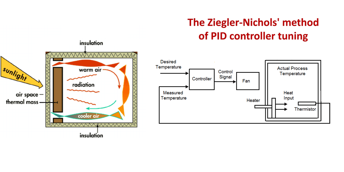
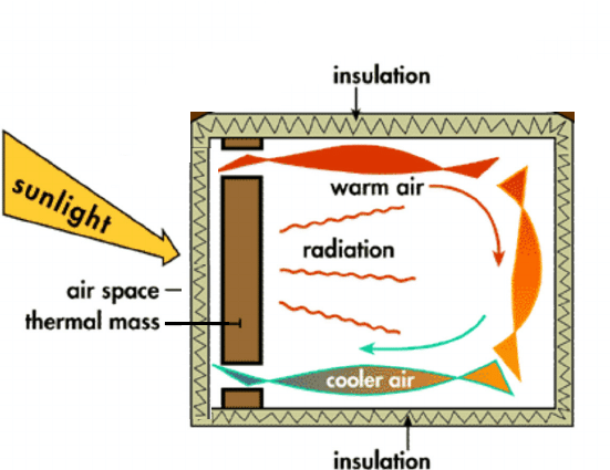
1) วงจรผลิตความร้อน (heater + room) ไม่ว่าจะเป็นตู้อบในอุตสาหกรรม (Oven) กระวบการผลิต หรือ กระบวนการทางเคมี ที่ต้องใช้ความร้อนจะมีลักษณะคล้ายๆ กันดังรูปที่ 1

เพื่อให้การวิเคราะห์เป็นไปโดยงาน เราจะลองเปลี่ยนกระบวนการให้ความร้อน เป็นบล๊อกไดอะแกรมจะได้ดังรูปที่ 2

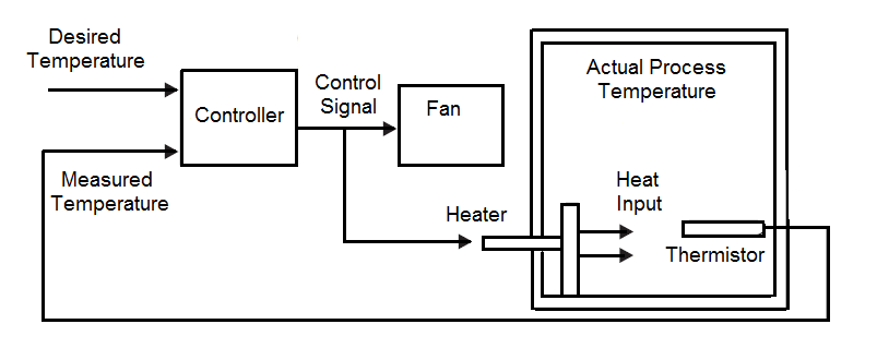
รูปที่ 2 Free body diagram ของระบบผลิตความร้อน

โดยปกติแล้วระบบก็จะประกอบไปด้วยตัวควบคุม (Controller) ตัวสร้างความร้อนและพัดลม(Heater +Fan) สัญญาณป้อนกลับหรือเซนเซอร์วัดอุณหภูมิ บริเวณทำความร้อนก็มักจะหุ้มด้วยฉนวน เพื่อความง่ายในการวิเคราะห์เราก็มักจะสมมติไว้ก่อนว่าระบบไม่มีการสูญเสียความร้อน (Adiabatic system) ไม่มีการแพร่รังสีความร้อน (Radiation)

2) ทำการทดสอบระบบแบบ Open Loop โดยขณะทดสอบมีอุณหภูมิโดยรอบ 34^oC ตั้งคำสั่งให้เตาอบทำอุณหภูมิ 92^oC จากการตรวจสอบวงจรเพาเวอร์ของ Heater ปรากฎว่าเมื่อมีคำสั่งทำอุณหภูมิ 92^oC มีแรงดันไฟฟ้าคำสั่งมายังวงจรผลิตความร้อน 0.5V นอกจากนี้ยังพบว่าเซนเซอร์วัดอุณหภูมิ ใช้ไอซีเบอร์ AD590 จากข้อมูลบน google.com พบว่าจะให้แรงดัน 10mV/^oC

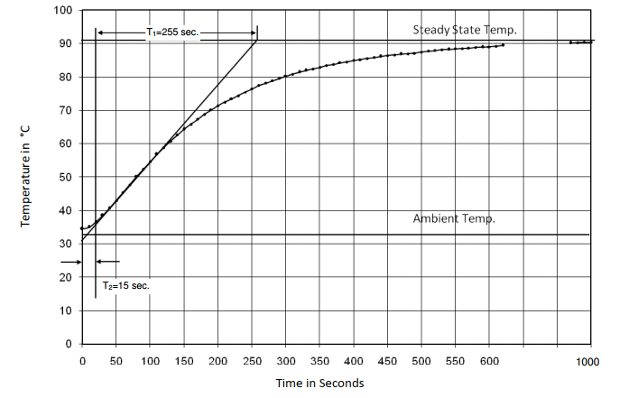
ไฟล์ผลการทดลองจริงถูกบันทึกอยู่ในรูป Excel โดยใช้ไฟล์ชื่อ open-loop-jan-24-correct.xlsx (ทดสอบตอนอุณหภูมิสภาพแวดล้อม 23^oC เพิ่มไปถึง 75^oC

3) จากบล๊อกก่อนหน้า Ziegler-Nichols วิธีที่ 1 ปรับแต่ง PID Controller โดยไม่ต้องทราบ สมการพลศาสตร์ของระบบ ทำให้สามารถคำนวณหาพารามิเตอร์ได้ดังนี้

คำนวณอัตราขยายของระบบตั้งค่าอุณหภูมิ (Set point) และระบบไฟฟ้ากำลังในการผลิตความร้อน ดังนี้

\(K=\frac{Final Temp. Oven – Ambient Temp.}{Input(Volts)}\)

(1)

\(K_{p}=\left ( \frac{1.2}{K} \right )\cdot \frac{T_{1}}{T_{2}}\)

(2)

\(T_{i}=2.0T_{2}\)

\(K_{i}=\frac{1}{T_{i}}\)

(3)

\(K_{d}=0.5T_{2}\)

(4)

จากประสบการณ์ของผู้เขียนพบว่า \(K_{d}\) อาจจะเป็นสาเหตุให้วงจรไฟฟ้ากำลังที่จ่ายกระแสให้ Heater สูงมาก เพื่อชะลอผลดังกล่าวผู้เขียนแนะนำให้ทดลองปรับค่าที่คำนวณได้อยู่ในช่วง 3-4 เท่า เช่นถ้าคำนวณ Kd=7.5 อาจจะใช้ค่า Kd=25 แทนก่อน แล้วค่อยๆ ปรับลดลงมา

3.1) ทำการคำนวณหาค่า K , T₁ และ T₂ จากไฟล์ผลการทดลอง open-loop-jan-24-correct.xlsx ตามคำสั่งดังนี้

clc, clearvars, close all;
% ritual to remove all the previous terminal output, vars, plots

f = xlsread('open-loop-jan-24-correct.xlsx', 'Sheet1', 'B2:B183');
n = size(f,1);
t = xlsread('open-loop-jan-24-correct.xlsx', 'Sheet1', 'A2:A183');

time_gap = 5;
[m, c, inflexion_point_idx] = findInflex(f, n, time_gap);
% m = inflex_slope
% c = inflex_yIntercept

% plotting
% main data
plot(t,f);
hold on;
% inflexion line
x = [ (f(1)-c)/m, (f(n)-c)/m ]; % T2 = x(1), T1 = x(2) - x(1)
y = m*x + c;
plot(x, y);
hold on;
% ambient line
plot( [0, (f(1)-c)/m], [f(1), f(1)] );
hold on;
% steady state line
plot( [(f(n)-c)/m, t(end)], [f(n), f(n)] );
hold on;
plot( time_gap*(inflexion_point_idx - 1), f(inflexion_point_idx) , 'g*');
title('Open loop response');
xlabel('time in s');
ylabel('temperature in degree C');

% const calculation
input_volts = 0.5;
K = ( f(n) - f(1) )/input_volts;
T2 = x(1);
T1 = x(2) - x(1);

% Writing to a file
fileID = fopen('open_loop_const.txt', 'w');
fprintf(fileID, '%f\n%f\n%f\n', K, T1, T2);
fclose(fileID);

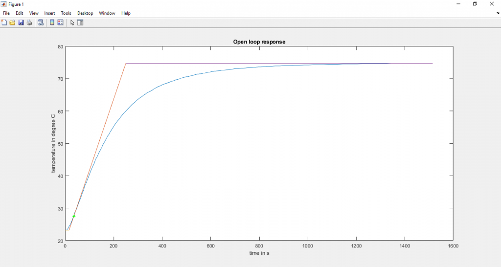
จะได้ผลลัพธ์เป็นไฟล์ open_loop_const.txt ซึ่งเก็บค่า K , T₁ และ T₂ และได้กราฟผลตอบสนองแบบ Open Loop ดังนี้

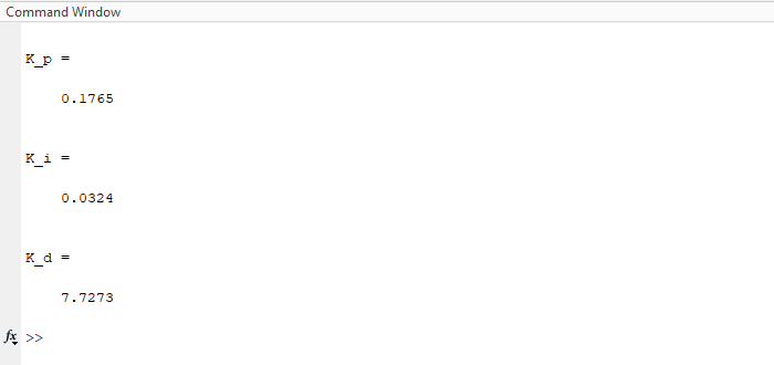
3.2) ทำการคำนวณค่าพารามิเตอร์ของ PID Controller โดยคำสั่งดังนี้

% fetching data of system parameters
open_loop_plot;
clc, clearvars, close all; % ritual to erase all the previous terminal message, vars, plots
fileID = fopen('open_loop_const.txt', 'r');
parameters = fscanf(fileID, '%f');
K = parameters(1);
T1 = parameters(2);
T2 = parameters(3);
fclose(fileID);

% p setting
K_p = ( 1.2*T1 )/( K*T2 );
K_pmax = 0.2;
p = (K_p/K_pmax);

% i setting
K_i = 1/( 2*T2 );
K_imax = 1/28;
i = K_i/K_imax;

% d setting
K_d = 0.5*T2;
K_dmax = 23.5;
d = K_d/K_dmax;

จะได้ผลลัพธ์จากการคำนวณดังนี้

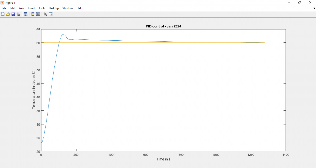
3.3) นำค่าที่คำนวณได้ไปใช้ และทดสอบระบบผลิตความร้อนที่ทำงานร่วมกับตัวควบคุมพีไอดี ตั้งอุณหภูมิที่ต้องการไว้ที่ 60^oC

ไฟล์ผลการทดลองถูกบันทึกอยู่ในรูป Excel โดยใช้ไฟล์ชื่อ pid-control-jan24.xlsx

ทำการพล๊อตกราฟผลการทำลองด้วยคำสั่งดังนี้

% temperature setpoint
set_val = 60;

% load data
f = xlsread('pid-control-jan24.xlsx', 'Sheet1', 'B2:B63');
t = xlsread('pid-control-jan24.xlsx', 'Sheet1', 'A2:A63');

% Plot dataset
plot(t,f);
hold on;
plot([t(1), t(end)], [f(1), f(1)]);
hold on;
plot([t(1), t(end)], [set_val, set_val]);
xlabel('Time in s');
ylabel('Temperature in degree C');
title('PID control - Jan 2024');

% peak overshoot computation
peak_overshoot = ( max(f) - f(end) )*100/f(end);

จะได้กราฟผลตอบสนองของระบบเมื่อมี PID Controller ดังนี้